Structured Temporal Inference in Hybrid State-Space Models

Hamidreza Hashempoor • Institute for AI, University of Stuttgart

Introduction Model Equations Inference Empirics

Introduction

Graphical model of Pi-SSM — Figure 1. Hybrid graph structure with continuous states and sampled discrete modes.

Real-world temporal systems are often hybrid: they evolve smoothly most of the time, then switch regimes under discrete events. Classical SLDS-style methods are principled but often require explicit Markov edges in the discrete chain and can become expensive when inference needs global sequence-level updates. Pi-SSM is designed to keep the useful structure of state-space inference while allowing local, state-conditioned mode selection.

The central modeling choice is to infer the mode directly from the latent trajectory signal, using $q(z_t \mid \mathbf{x}_{t-1})$. This avoids forcing a hard coded transition prior of the form $p(z_t \mid z_{t-1})$, and enables online operation in which each step is updated with local information rather than global backward passes.

To preserve numerical structure, Pi-SSM keeps a Kalman-like update template for the continuous posterior but uses a learned, positive-definite surrogate for the inversion-like component. This provides flexibility without abandoning filtering algebra.

Model Factorization

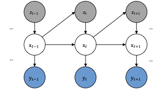
Factor-graph interpretation — Figure 2. Factor-graph view motivating local message updates over $(\mathbf{x}_t, z_t)$.

We model trajectories with continuous latent states $\mathbf{x}_{1:T}$, discrete modes $z_{1:T}$, and observations $\mathbf{y}_{1:T}$. The joint distribution is factorized as

$$ p(\mathbf{x}_{1:T}, z_{1:T}, \mathbf{y}_{1:T}) = p(\mathbf{x}_0) \prod_{t=1}^{T} p(z_t \mid \mathbf{x}_{t-1}) p(\mathbf{x}_t \mid \mathbf{x}_{t-1}, z_t) p(\mathbf{y}_t \mid \mathbf{x}_t, z_t). $$

This state-dependent discrete factorization is the key structural difference relative to Markov-mode SLDS.

At each step, the filtered approximation is represented as

$$ q(\mathbf{x}_t \mid \mathbf{y}_{1:t}) = \mathcal{N}\!\left(\hat{\boldsymbol{\mu}}_{t\mid t},\, \hat{\boldsymbol{\Sigma}}_{t\mid t}\right), \qquad z_t \sim q(z_t \mid \mathbf{x}_{t-1}). $$

This decomposition supports local updates in time while retaining a probabilistic interpretation for both state and mode variables.

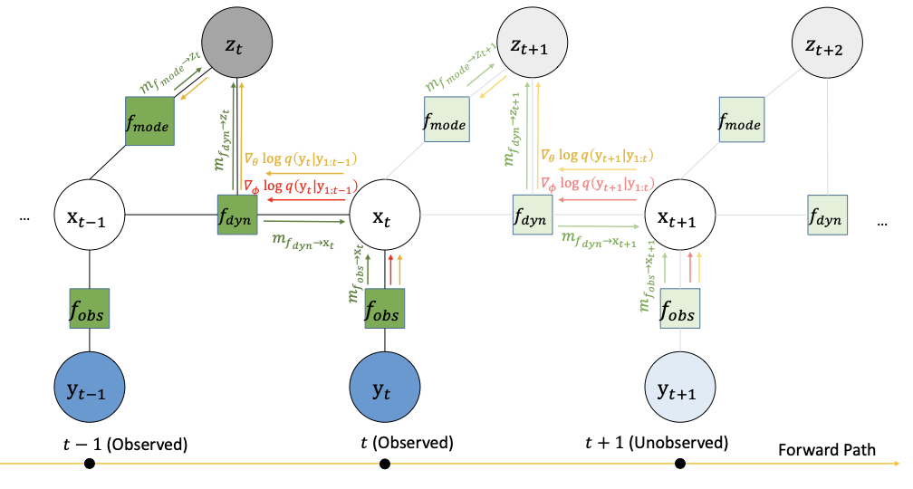
Nested Inference and Updates

Continuous updates follow a pseudo-Kalman form with a learned gain parameterization:

$$ \hat{\mathbf{K}}_t = \hat{\boldsymbol{\Sigma}}_{t\mid t-1}\mathbf{C}_{z_t}^{\top}\mathbf{L}_t\mathbf{L}_t^{\top}, \qquad \mathbf{L}_t = \mathrm{RNN}\!\left([\hat{\boldsymbol{\Sigma}}_{t\mid t-1}, \mathbf{r}_t]\right). $$

$$ \hat{\boldsymbol{\mu}}_{t\mid t} = \hat{\boldsymbol{\mu}}_{t\mid t-1} + \hat{\mathbf{K}}_t\left(\mathbf{y}_t - \mathbf{C}_{z_t}\hat{\boldsymbol{\mu}}_{t\mid t-1}\right), $$ $$ \hat{\boldsymbol{\Sigma}}_{t\mid t} = \hat{\boldsymbol{\Sigma}}_{t\mid t-1} + \hat{\mathbf{K}}_t\left(\mathbf{C}_{z_t}\hat{\boldsymbol{\Sigma}}_{t\mid t-1}\mathbf{C}_{z_t}^{\top}+\mathbf{R}_t\right)\hat{\mathbf{K}}_t^{\top}. $$

The gain keeps the structure of filtering while replacing unstable inverse terms with a learned PSD factor.

A compact message-passing approximation for beliefs can be summarized as

$$ \operatorname{Belief}(\mathbf{x}_t) \propto m_{f_{\mathrm{dyn}}\to\mathbf{x}_t} \cdot m_{f_{\mathrm{obs}}\to\mathbf{x}_t} \cdot m_{f_{\mathrm{mode}}\to\mathbf{x}_t}, $$ $$ \operatorname{Belief}(z_t) \propto m_{f_{\mathrm{dyn}}\to z_t} \cdot m_{f_{\mathrm{mode}}\to z_t}. $$

For training, we optimize predictive likelihood terms with local discrete-variable gradients. One practical objective is a rolling negative log-likelihood:

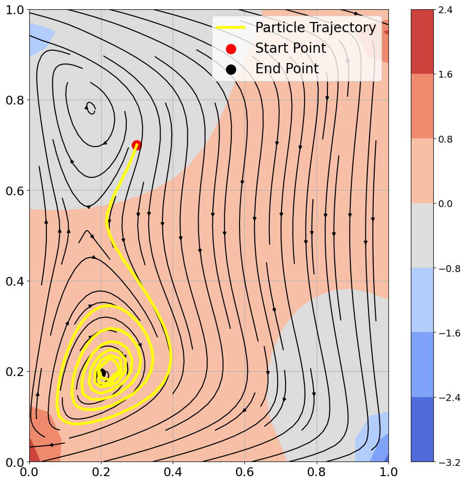
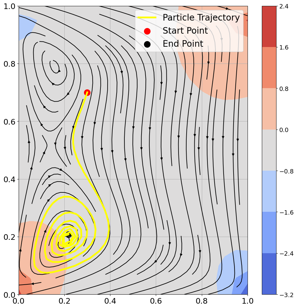
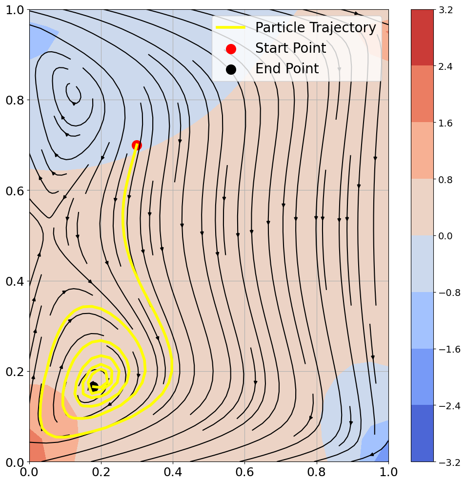
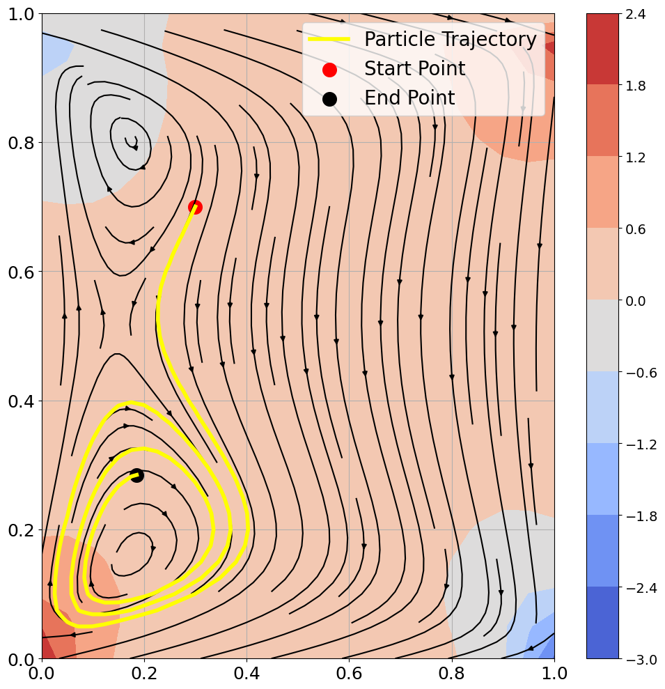
$$ \mathcal{L}(\theta,\phi) = -\sum_{t=1}^{T}\log q\!\left(\mathbf{y}_t \mid \mathbf{y}_{1:t-1};\theta,\phi\right), $$ $$ \nabla_\theta \mathcal{L} \approx -\sum_{t=1}^{T} \mathbb{E}_{z_t\sim q_\theta(z_t\mid\mathbf{x}_{t-1})} \left[ \log q_\phi(\mathbf{y}_t\mid z_t,\mathbf{x}_{t-1})\,\nabla_\theta\log q_\theta(z_t\mid\mathbf{x}_{t-1}) \right]. $$

Empirical Behavior

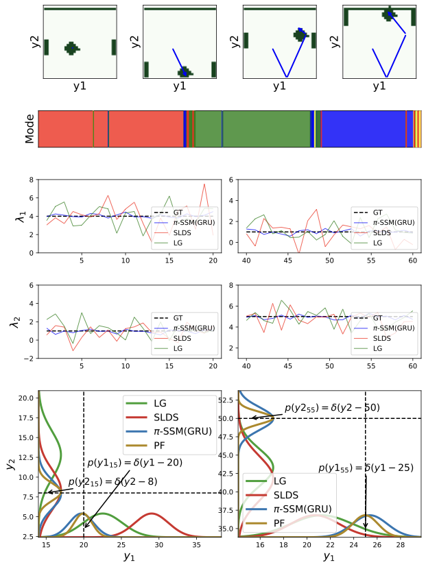
Pong experiment figure — Figure 3. Pong analysis: mode evolution, transition-spectrum dynamics, and predictive uncertainty near collision events.

In Pong, regime changes align with contact events and are visible in both learned discrete assignments and transition-spectrum shifts. The state-conditioned mode predictor captures these transitions without explicit $p(z_t\mid z_{t-1})$ persistence terms.

Across tasks, we observe three consistent behaviors:

Reliable tracking under hybrid continuous-discrete dynamics.
Stable recursive updates from the learned gain factorization.
Practical online inference without full-sequence backtracking.

Navier ground-truth-like panel — Figure 4. Qualitative comparison on Navier-Stokes-type dynamics.

Navier Pi-SSM panel — Figure 4. Qualitative comparison on Navier-Stokes-type dynamics.