AISTATS 2026 Batch • Paper 5

16 minute read

Published: July 2026

Gaussian Equivalence for Self-Attention Spectra

Hamidreza Hashempoor • Institute for AI, University of Stuttgart

← Back to series Original paper ↗ View notebook Download .ipynb Experiment Results

The idea Attention setup Normalizer & $f$ Gaussian equivalence Seven models Experiment Results Notebook

What does the singular-value spectrum of a freshly-initialized softmax self-attention matrix actually look like? The surprising answer: strip off one rank-one spike and what remains is, to leading order, the spectrum of a simple linear Gaussian matrix. This post follows Gaussian Equivalence for Self-Attention Spectra and verifies its central claim empirically: in the high-dimensional limit the centered, scaled attention matrix $\sqrt{\ell}\,(A-u_\ell u_\ell^\top)$ has the same bulk squared-singular-value distribution as an explicit Gaussian-equivalent linear model. The whole story is checked on a $d=1000$ experiment whose numbers are reproduced by the companion notebook.

The idea: attention = a rank-one mode + a Gaussian bulk

Softmax attention is nonlinear and its rows are coupled through a shared normalizer, so its spectrum has no business being simple. Yet in the proportional high-dimensional regime a clean decomposition emerges. The attention matrix splits into a rank-one uniform-averaging mode — every row is nearly the uniform distribution, contributing a single large Perron singular value — plus a small diffusive fluctuation whose bulk spectral law is deterministic and matches that of a purely linear random matrix.

The claim in one line. Write $A$ for softmax attention and $u_\ell u_\ell^\top$ for the uniform (rank-one) attention. Then $A\approx u_\ell u_\ell^\top+\tfrac{1}{\sqrt{\ell}}\,Y_{\text{bulk}}$, and the bulk $Y_{\text{bulk}}$ has the same limiting squared-singular-value distribution as the Gaussian-equivalent linear model $Y_{\text{lin}}^f=\beta\,\tfrac{S}{\sqrt d}+\sqrt{e^{\beta^2}-1-\beta^2}\,\tfrac{W}{\sqrt d}$, with $S$ the attention score matrix and $W$ an independent Gaussian. The nonlinearity survives only through two scalar constants.

The attention matrix

Take an input sequence $X\in\mathbb R^{\ell\times d}$, query/key weights $W^Q,W^K\in\mathbb R^{d\times d_{qk}}$ with i.i.d. $\mathcal N(0,1)$ entries, and form the score matrix $S=\tfrac{1}{\sqrt{d_{qk}}}\,XW^Q(W^K)^\top X^\top$. The experiment uses the clean reduction $\ell=d=d_{qk}$ and $X=I_d$, so the score matrix is simply

$$ S=\frac{1}{\sqrt{d}}\,W^Q(W^K)^\top . $$

Softmax over each row gives the row-stochastic attention matrix, and the uniform baseline is its rank-one mean:

$$ A=\operatorname{softmax}(\beta S),\quad A_{ij}=\frac{e^{\beta S_{ij}}}{Z_i},\quad Z_i=\sum_j e^{\beta S_{ij}};\qquad u_d u_d^\top=\frac1d\mathbf 1\mathbf 1^\top,\quad u_d=\frac{1}{\sqrt d}\mathbf 1. $$

The object of interest is the centered fluctuation around the uniform mode,

$$ A_\perp = A - u_d u_d^\top , $$

where $\beta>0$ is an inverse-temperature. All the action is in $A_\perp$: the uniform mode $u_d u_d^\top$ carries the one big singular value, and $A_\perp$ carries the bulk.

The deterministic normalizer and the nonlinearity $f$

The row normalizers $Z_i$ are what make attention rows dependent. The key simplification is that for large $d$ they concentrate: since each $S_{ij}\approx\mathcal N(0,1/d)\cdot\sqrt d$ behaves like a standard Gaussian $\chi$, the law of large numbers gives

$$ Z_i \;\approx\; d\,\mathbb E\!\left[e^{\beta\chi}\right] \;=\; d\,e^{\beta^2/2},\qquad \chi\sim\mathcal N(0,1). $$

Replacing $Z_i$ by this deterministic value turns each entry into a pointwise nonlinearity of the score:

$$ A_{ij}\approx\frac1d\,e^{\beta S_{ij}-\beta^2/2}=\frac1d\bigl(1+f(S_{ij})\bigr),\qquad f(x)=e^{\beta x-\beta^2/2}-1, $$

so that the centered, scaled fluctuation is governed entirely by $f$ applied to the scores:

$$ \sqrt d\,(A-u_du_d^\top)\;\approx\;\frac{1}{\sqrt d}\,f(S). $$

The function $f$ is centered ($\mathbb E[f(\chi)]=0$) and, remarkably, its whole spectral effect is summarized by just two scalars — a linear coefficient and a variance:

$$ \theta_1=\mathbb E\!\left[f(\chi)^2\right]=e^{\beta^2}-1,\qquad \theta_2=\bigl(\mathbb E[f'(\chi)]\bigr)^2=\beta^2, $$

The convexity inequality $e^{x}\ge 1+x$ gives $\theta_1\ge\theta_2$, with equality only at $\beta=0$; $\theta_1-\theta_2=e^{\beta^2}-1-\beta^2\ge 0$ is exactly the non-linear "residual" energy that a linear model cannot capture with the score alone.

The Gaussian-equivalent linear model

Here is the heart of the result. By an orthogonal (Stein) projection, the scalar random variable $f(\chi)$ can be split into the part correlated with $\chi$ plus an independent Gaussian residual carrying the leftover variance:

$$ f(\chi)\;\approx\;\sqrt{\theta_2}\;\chi\;+\;\sqrt{\theta_1-\theta_2}\;\eta,\qquad \eta\sim\mathcal N(0,1),\ \eta\perp\chi. $$

Promoting this to matrices — the score $S/\sqrt d$ plays the role of $\chi$, and an independent Gaussian $W/\sqrt d$ plays the role of $\eta$ — turns the nonlinear $f(S)/\sqrt d$ into a linear surrogate. With the exact statistics of $f$ this is the Gaussian-equivalent model:

$$ \boxed{\;Y_{\text{lin}}^f=\beta\,\frac{S}{\sqrt d}\;+\;\sqrt{\,e^{\beta^2}-1-\beta^2\,}\,\frac{W}{\sqrt d}\;} $$

This is not an entrywise equality — the two matrices are entirely different objects. It is an asymptotic statement about their bulk singular-value distributions. In the proportional regime $d,\ell,d_{qk}\to\infty$ with $\ell/d\to\gamma$ and $d_{qk}/d\to\psi$, the theory shows two things:

Rank-one dominance: $s_1(A)\to 1$ almost surely — the top singular value is exactly the uniform Perron mode, nothing else.
Bulk equivalence: the squared-singular-value law of $\sqrt\ell\,A_\perp$ converges to the same limiting law $\nu_\infty(\beta,\gamma,\psi)$ as that of $Y_{\text{lin}}^f$.

Together these give the practical decomposition advertised in the introduction,

$$ A\;\approx\;u_\ell u_\ell^\top\;+\;\frac{1}{\sqrt\ell}\,Y_{\text{bulk}}, $$

a rank-one averaging mode plus a diffusive bulk with a deterministic spectral law.

A polynomial bridge

To connect the true nonlinearity to its linear surrogate the paper interposes a polynomial model: replace $e^{(\cdot)}$ by its truncated Taylor expansion $P_n(x)=\sum_{k

$$ Q_n(x)=e^{-\beta^2/2}\bigl(P_n(\beta x)-\mathbb E[P_n(\beta\chi)]\bigr),\qquad n_d=\Bigl\lceil c\,\frac{\log d}{\log\log d}\Bigr\rceil. $$

$Q_n$ has its own statistics $\theta_1^Q=\mathbb E[Q_n(\chi)^2]$ and $\theta_2^Q=(\mathbb E[Q_n'(\chi)])^2$ (estimated by Monte-Carlo), and its own Gaussian-equivalent $Y_{\text{lin}}^Q=\sqrt{\theta_2^Q}\,S/\sqrt d+\sqrt{\theta_1^Q-\theta_2^Q}\,W/\sqrt d$. As the degree grows, $Q_n\to f$ and the two equivalences coincide.

A ladder of seven models

The experiment builds seven matrices that step from the true attention down to the linear Gaussian equivalent. Comparing their bulk spectra shows the equivalence tighten rung by rung.

#	Name	Definition	Role
M0	`sqrt_d_A`	$\sqrt d\,A$	reference; keeps the rank-one outlier
M1	`sqrt_d_A_perp`	$\sqrt d\,(A-u_du_d^\top)$	cleanest target for the theorem
M2	`Y`	$e^{\beta S}/(e^{\beta^2/2}\sqrt d)$	deterministic-normalizer exponential
M3	`Y_f`	$f(S)/\sqrt d$	centered nonlinear model
M4	`Y_Q`	$Q_n(S)/\sqrt d$	polynomial (Taylor) approximation
M5	`Y_Q_lin`	$\sqrt{\theta_2^Q}\tfrac{S}{\sqrt d}+\sqrt{\theta_1^Q-\theta_2^Q}\tfrac{W}{\sqrt d}$	Gaussian-equivalent of $Q_n$
M6	`Y_f_lin`	$\beta\tfrac{S}{\sqrt d}+\sqrt{e^{\beta^2}-1-\beta^2}\,\tfrac{W}{\sqrt d}$	final Gaussian-equivalent, exact $\theta$

The experiment

A single high-dimensional draw is already enough to see the limiting behaviour. The reported run averages over $10$ independent trials at $d=1000$; each trial draws fresh Gaussian $W^Q,W^K,W$, builds all seven models, and compares their squared-singular-value bulk (after discarding the top $3$ values, which hold any rank-one spikes) against the cleanest reference sqrt_d_A_perp.

Setting	Value	Setting	Value
dimensions $d=\ell=d_{qk}$	1000	input $X$	$I_d$ (identity)
inverse temp. $\beta$	1.0	trials	10
top-$k$ removed (bulk)	3	dtype	float64
polynomial $c$	2.0 → degree $n_d=8$	$\theta^Q$ MC samples	200,000
histogram bins	120 over $[0,8]$	SVD	full, dense

Results

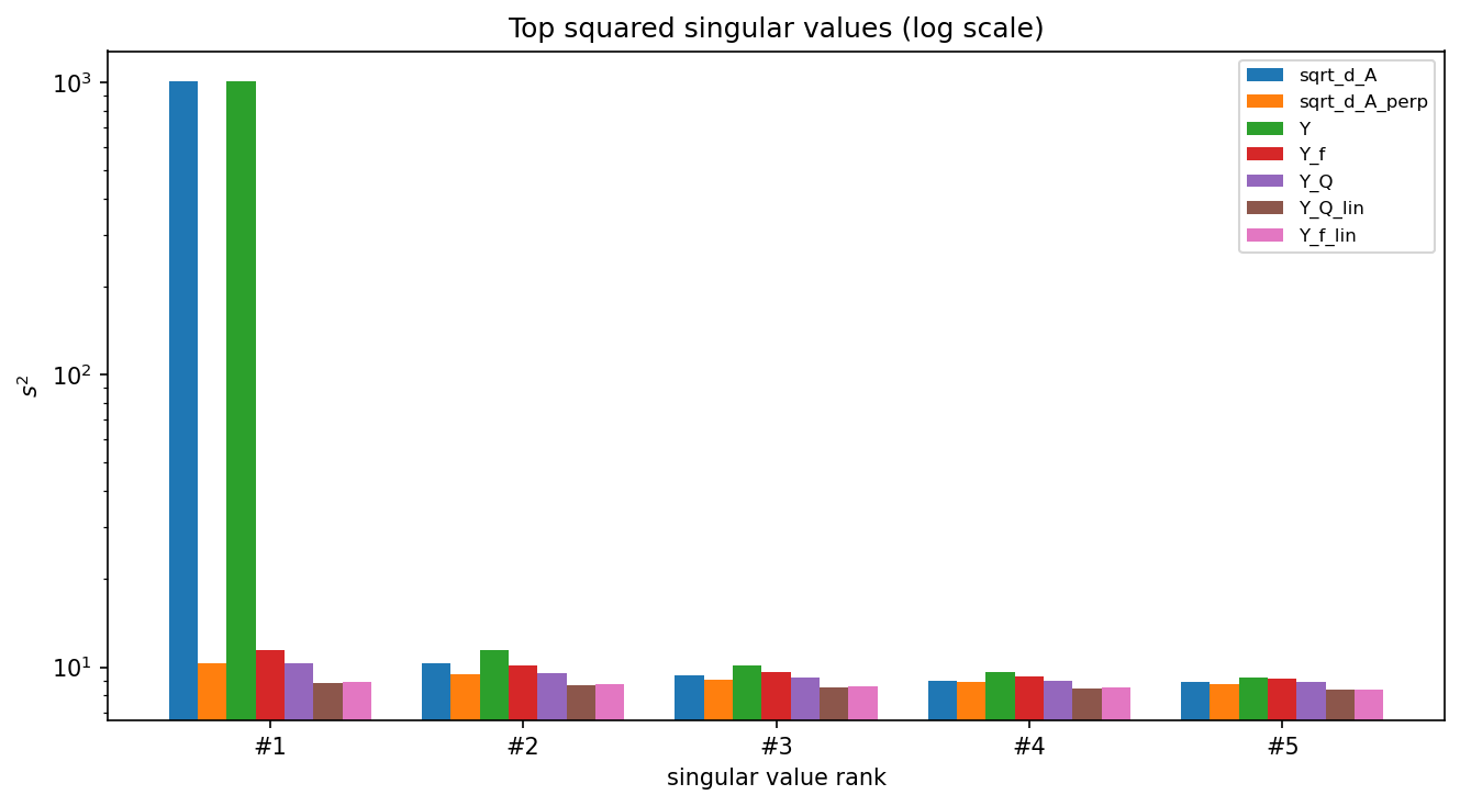
All three theoretical claims come out cleanly at $d=1000$. First, the rank-one mode: the top squared singular value of $\sqrt d\,A$ (and of the deterministic-normalizer model $Y$) sits at $\sim\!1000$, while every centered/linear model has no such spike — its largest bulk value is only $\sim\!10$.

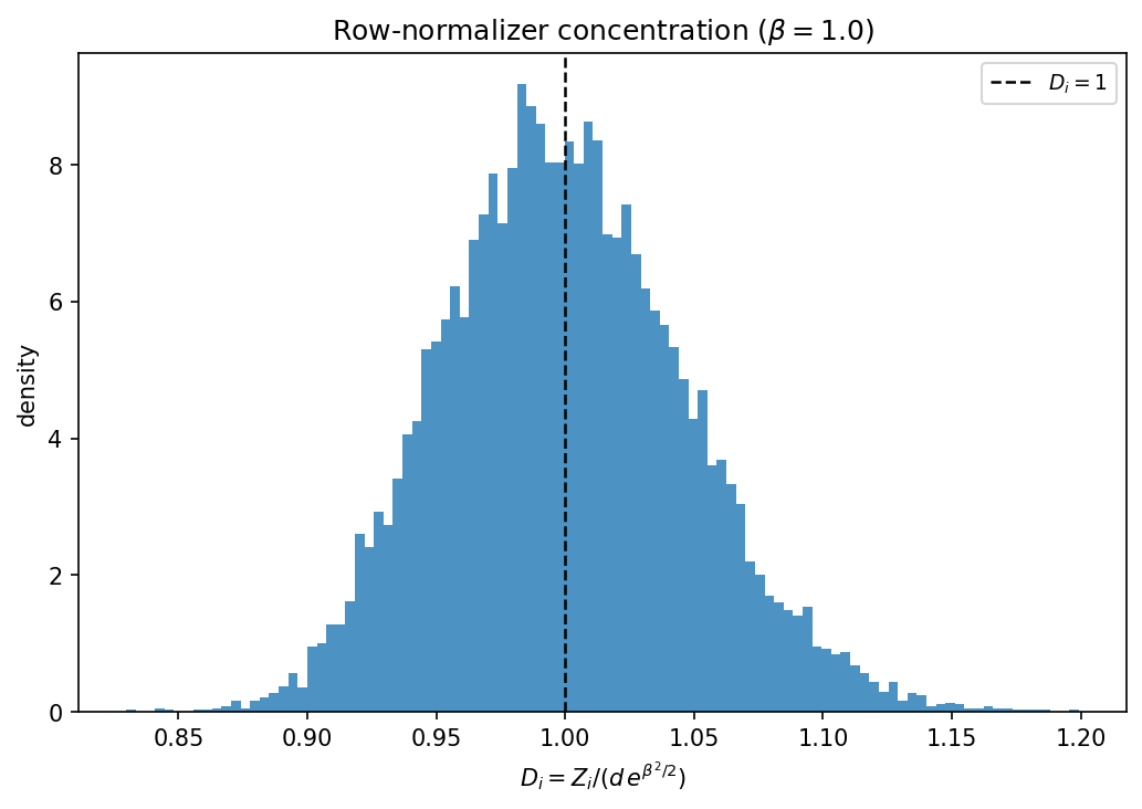
Bar chart of the top five squared singular values per model on a log scale; sqrt_d_A and Y show a spike near 1000 while all other models sit near 10. — Figure 1. Top-5 squared singular values per model (log scale, averaged over 10 trials). **sqrt_d_A** and Y carry the rank-one Perron spike $s_1^2\approx1000\approx d$; removing the uniform mode (**sqrt_d_A_perp**) or working with any centered/linear model drops $s_1^2$ to $\sim\!10$ — the outlier is *entirely* the uniform-averaging direction.

Second, the deterministic-normalizer approximation that everything rests on. The diagnostic $D_i=Z_i/(d\,e^{\beta^2/2})$ concentrates tightly at $1$ (mean $0.99994$, std $0.047$, worst-case deviation $0.199$ across all $10^4$ rows) — exactly what licenses replacing $Z_i$ by $d\,e^{\beta^2/2}$.

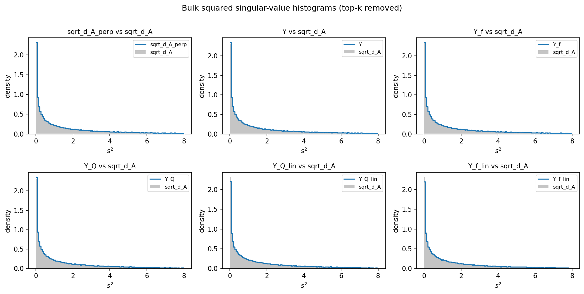
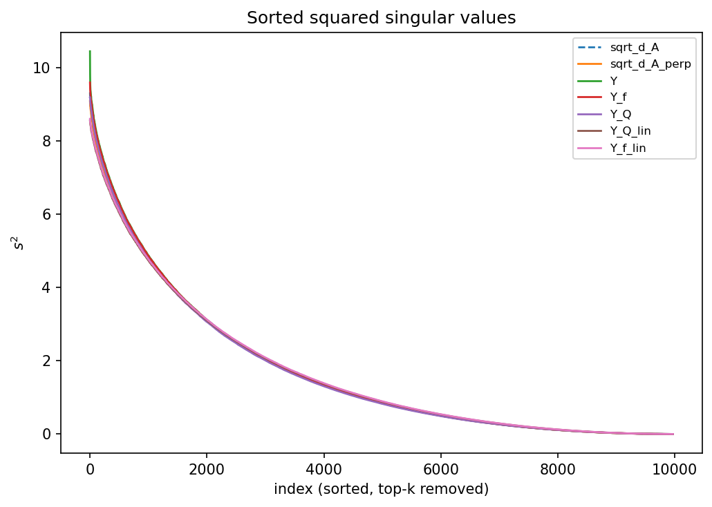
Histogram of the row-normalizer diagnostic D_i, sharply peaked at 1. — Figure 2. Row-normalizer concentration: histogram of $D_i=Z_i/(d\,e^{\beta^2/2})$ over all rows and trials. Tightly peaked at the dashed line $D_i=1$, validating $Z_i\approx d\,e^{\beta^2/2}$ at finite $d$.

Third — the main event — bulk spectral equivalence. Once the top-3 values are removed, the squared-singular-value histograms of the nonlinear models and their linear Gaussian equivalents line up, and the sorted-curve overlay is nearly a single line.

Grid of six panels, each overlaying a model's bulk squared-singular-value histogram on the reference sqrt_d_A histogram. — Figure 3. Bulk squared-singular-value histograms (top-3 removed), each model (blue step) vs. the reference **sqrt_d_A** bulk (grey). The polynomial model **Y_Q** and the Gaussian-equivalent **Y_f_lin** track the reference bulk closely; small tail differences are the expected finite-$d$ gap, since the equivalence is asymptotic.

Overlaid descending sorted bulk squared-singular-value curves for all seven models; the curves nearly coincide. — Figure 4. Sorted (descending) bulk squared singular values for all seven models. The reference **sqrt_d_A** is dashed; every other curve nearly coincides across the bulk — the visual statement of a shared limiting spectral law.

Representative numbers

The diagnostics and bulk distances from the reported 10-trial run:

Model	top-1 $s^2$	$L_1$ to `sqrt_d_A_perp`	Wasserstein	mean curve err
`sqrt_d_A`	1002.21	0.0202	0.0068	0.0068
`sqrt_d_A_perp`	10.29	0.0000	0.0000	0.0000
`Y`	1004.40	0.0320	0.0313	0.0313
`Y_f`	11.48	0.0322	0.0265	0.0265
`Y_Q`	10.28	0.0381	0.0165	0.0165
`Y_Q_lin`	8.83	0.0486	0.0352	0.0352
`Y_f_lin`	8.88	0.0501	0.0389	0.0389

Statistics ($\beta=1$): $\theta_1(f)=e-1=1.7183$, $\theta_2(f)=1.0$; Monte-Carlo polynomial $\theta_1^Q=1.7047$, $\theta_2^Q=0.9987$ (degree $n_d=8$). Rank-one diagnostics: mean $s_1(A)=1.0011$ and mean $s_1(\sqrt d\,A)=31.658$ vs. $\sqrt{1000}=31.623$. Normalizer: mean $0.99994$, std $0.047$, max $|D_i-1|=0.199$.

Reading the three regimes of the ladder. (1) Rank-one: only sqrt_d_A and Y keep the $s_1^2\approx d$ spike; centering removes it and confirms it is the uniform mode. (2) Nonlinear vs. deterministic-normalizer: Y and Y_f match sqrt_d_A_perp closely, so the normalizer approximation costs almost nothing. (3) Linear surrogate: the Gaussian-equivalents Y_Q_lin and Y_f_lin sit a hair further from the reference than the polynomial Y_Q — the residual is the finite-$d$ gap that shrinks as $d\to\infty$. In every case the bulk distances are small and of the same order, which is the empirical content of the theorem.

The takeaway: a randomly-initialized softmax attention map is spectrally boring in the best possible way. One rank-one averaging direction aside, its singular values behave like those of a linear Gaussian matrix whose only memory of the softmax is two numbers, $\theta_1$ and $\theta_2$.

Reproduce it

The companion notebook rebuilds the whole experiment from scratch with only numpy (and matplotlib for the figures). It constructs the score matrix, the softmax attention, the nonlinearity $f$, the Taylor polynomial $Q_n$, and both Gaussian-equivalent models, then computes singular-value spectra, the normalizer diagnostic, and the bulk histogram distances — printing the exact $\theta$ statistics and diagnostics reported above. It runs $5$ trials by default (rather than $10$) for a snappier execution; this only smooths the Monte-Carlo histograms and leaves the verified quantities unchanged.

View notebook (rendered) Download .ipynb