Synthetic-Regularized Kernel Regression — Minimal Reproduction
A minimal, numpy-only reproduction of the 1-D experiment from the post. It
implements the estimator $\alpha=(K_N+N\lambda I)^{-1}(y+N\lambda\beta)$, the Monte-Carlo
bias² / variance / risk decomposition, and the spectral-discrepancy proxy. The printed
numbers match the reference values reported in the post to ~$10^{-9}$.
Setup
Only numpy is needed (plus matplotlib for the plot).
import numpy as np
np.set_printoptions(precision=4)SEED, N_TRAIN, N_TEST = 42, 64, 1000
NOISE_STD, REPETITIONS, PROJECTION_RIDGE, LENGTHSCALE = 0.1, 200, 1e-8, 0.15
LAMBDAS = [0.0003, 0.001, 0.003, 0.01, 0.03, 0.1, 0.3, 1.0, 3.0, 10.0]
GENERATORS = [
{"name": "perfect", "delta": 0.0},
{"name": "smooth_bias", "delta": 0.3},
{"name": "high_frequency_bias", "delta": 0.3, "frequency": 10},
]Target, data, kernel, generators
def f_star(x):
    x = np.asarray(x, dtype=np.float64)
    return np.sin(2.0 * np.pi * x) + 0.5 * np.cos(4.0 * np.pi * x)

def make_train_inputs(n, seed):
    rng = np.random.default_rng(seed)
    return np.sort(rng.uniform(0.0, 1.0, size=n))

def make_test_inputs(n):
return np.linspace(0.0, 1.0, n)def rbf_kernel(xa, xb, lengthscale):
xa = np.asarray(xa, dtype=np.float64).reshape(-1, 1)
xb = np.asarray(xb, dtype=np.float64).reshape(1, -1)
return np.exp(-((xa - xb) ** 2) / (2.0 * lengthscale ** 2))def evaluate_generator(name, x, delta=0.0, frequency=10):
base = f_star(x)
if name == "perfect":
return base
if name == "smooth_bias":
return base + delta * np.sin(2.0 * np.pi * x)
if name == "high_frequency_bias":
return base + delta * np.sin(2.0 * np.pi * frequency * x)
raise ValueError(f"Unknown generator: {name}")The estimator
def project_generator_to_kernel_span(K_train, g_train, ridge):
    n = K_train.shape[0]
    return np.linalg.solve(K_train + ridge * np.eye(n), g_train)

def fit_synthetic_krr(K_train, y_train, beta, lam):
    n = K_train.shape[0]
    lam_n = n * lam
    return np.linalg.solve(K_train + lam_n * np.eye(n), y_train + lam_n * beta)

def predict(K_test_train, alpha):
return K_test_train @ alphadef bias_variance_decomposition(predictions, y_true):
mean_pred = predictions.mean(axis=0)
bias2 = float(np.mean((y_true - mean_pred) ** 2))
variance = float(np.mean((predictions - mean_pred[None, :]) ** 2))
return bias2, variance, bias2 + varianceRun the sweep
Three generators × ten $\lambda$ values, 200 noise repetitions each, training inputs fixed.
x_train = make_train_inputs(N_TRAIN, SEED)
x_test = make_test_inputs(N_TEST)
y_true_train, y_true_test = f_star(x_train), f_star(x_test)
K_train = rbf_kernel(x_train, x_train, LENGTHSCALE)
K_test_train = rbf_kernel(x_test, x_train, LENGTHSCALE)

rng = np.random.default_rng(SEED + 1000)   # single stream drives all noise draws
results = {}
print(f"{'generator':<22}{'lambda':>9}{'bias2':>13}{'variance':>13}{'risk':>13}")
print('-' * 70)
for gen in GENERATORS:
    g_train = evaluate_generator(x=x_train, **gen)
    beta = project_generator_to_kernel_span(K_train, g_train, PROJECTION_RIDGE)
    for lam in LAMBDAS:
        preds = np.empty((REPETITIONS, N_TEST))
        for r in range(REPETITIONS):
            eps = rng.normal(0.0, NOISE_STD, size=N_TRAIN)
            alpha = fit_synthetic_krr(K_train, y_true_train + eps, beta, lam)
            preds[r] = predict(K_test_train, alpha)
        b2, v, risk = bias_variance_decomposition(preds, y_true_test)
        results[(gen['name'], lam)] = (b2, v, risk)
print(f"{gen['name']:<22}{lam:>9.4g}{b2:>13.4e}{v:>13.4e}{risk:>13.4e}")generator lambda bias2 variance risk ---------------------------------------------------------------------- perfect 0.0003 7.4549e-06 1.5827e-03 1.5901e-03 perfect 0.001 4.5299e-06 1.3356e-03 1.3401e-03 perfect 0.003 3.5072e-06 1.0557e-03 1.0592e-03 perfect 0.01 1.4574e-06 8.8872e-04 8.9018e-04 perfect 0.03 4.5421e-06 5.6287e-04 5.6741e-04 perfect 0.1 1.5004e-06 2.9375e-04 2.9525e-04 perfect 0.3 1.8378e-07 1.0750e-04 1.0769e-04 perfect 1 4.4351e-07 2.4887e-05 2.5331e-05 perfect 3 3.5098e-08 3.6897e-06 3.7248e-06 perfect 10 2.1743e-09 3.8032e-07 3.8249e-07 smooth_bias 0.0003 6.4654e-06 1.5609e-03 1.5673e-03 smooth_bias 0.001 2.5725e-05 1.3382e-03 1.3640e-03 smooth_bias 0.003 5.2263e-05 1.0638e-03 1.1161e-03 smooth_bias 0.01 1.5727e-04 8.8010e-04 1.0374e-03 smooth_bias 0.03 7.2752e-04 6.0237e-04 1.3299e-03 smooth_bias 0.1 3.7847e-03 2.7488e-04 4.0596e-03 smooth_bias 0.3 1.2344e-02 1.1816e-04 1.2462e-02 smooth_bias 1 2.7175e-02 2.1489e-05 2.7196e-02 smooth_bias 3 3.7439e-02 3.3636e-06 3.7442e-02 smooth_bias 10 4.2464e-02 3.7774e-07 4.2465e-02 high_frequency_bias 0.0003 7.0241e-02 1.5531e-03 7.1794e-02 high_frequency_bias 0.001 7.6681e-02 1.3240e-03 7.8005e-02 high_frequency_bias 0.003 8.3342e-02 1.0704e-03 8.4413e-02 high_frequency_bias 0.01 8.9639e-02 8.8015e-04 9.0519e-02 high_frequency_bias 0.03 9.3951e-02 5.6589e-04 9.4517e-02 high_frequency_bias 0.1 9.8418e-02 2.7131e-04 9.8689e-02 high_frequency_bias 0.3 1.0212e-01 1.0381e-04 1.0222e-01 high_frequency_bias 1 1.0607e-01 2.2957e-05 1.0609e-01 high_frequency_bias 3 1.0829e-01 4.0103e-06 1.0829e-01 high_frequency_bias 10 1.0940e-01 3.5784e-07 1.0940e-01
Spectral-discrepancy proxy
def discrepancy_proxy(K_train, f_star_train, g_train, n_train, eps=1e-12):
    evals, evecs = np.linalg.eigh(K_train / n_train)
    coeffs = evecs.T @ (f_star_train - g_train)
    return float(np.sum((coeffs ** 2) / (evals + eps) ** 2))

print('Spectral discrepancy proxy  D_hat(f*, g)^2 :')
for gen in GENERATORS:
    g_train = evaluate_generator(x=x_train, **gen)
    d = discrepancy_proxy(K_train, y_true_train, g_train, N_TRAIN)
print(f" {gen['name']:<22} {d:.4e}")Spectral discrepancy proxy D_hat(f*, g)^2 : perfect 0.0000e+00 smooth_bias 2.2422e+11 high_frequency_bias 8.7433e+23
The discrepancy ranks the generators exactly as the risk does: perfect ($0$) < smooth ($\sim10^{11}$) < high-frequency ($\sim10^{23}$). Mismatch in the small-eigenvalue directions is what the $1/\mu_j^2$ weighting punishes.
Plot: risk vs. $\lambda$
import matplotlib.pyplot as plt

fig, ax = plt.subplots(figsize=(6.4, 4.2))
for gen in GENERATORS:
    name = gen['name']
    risks = [results[(name, lam)][2] for lam in LAMBDAS]
    ax.loglog(LAMBDAS, risks, marker='o', label=name)
ax.set_xlabel(r'regularization strength $\lambda$')
ax.set_ylabel('population risk')
ax.set_title('Risk vs. lambda')
ax.legend(); ax.grid(True, which='both', alpha=0.3)
fig.tight_layout(); plt.show()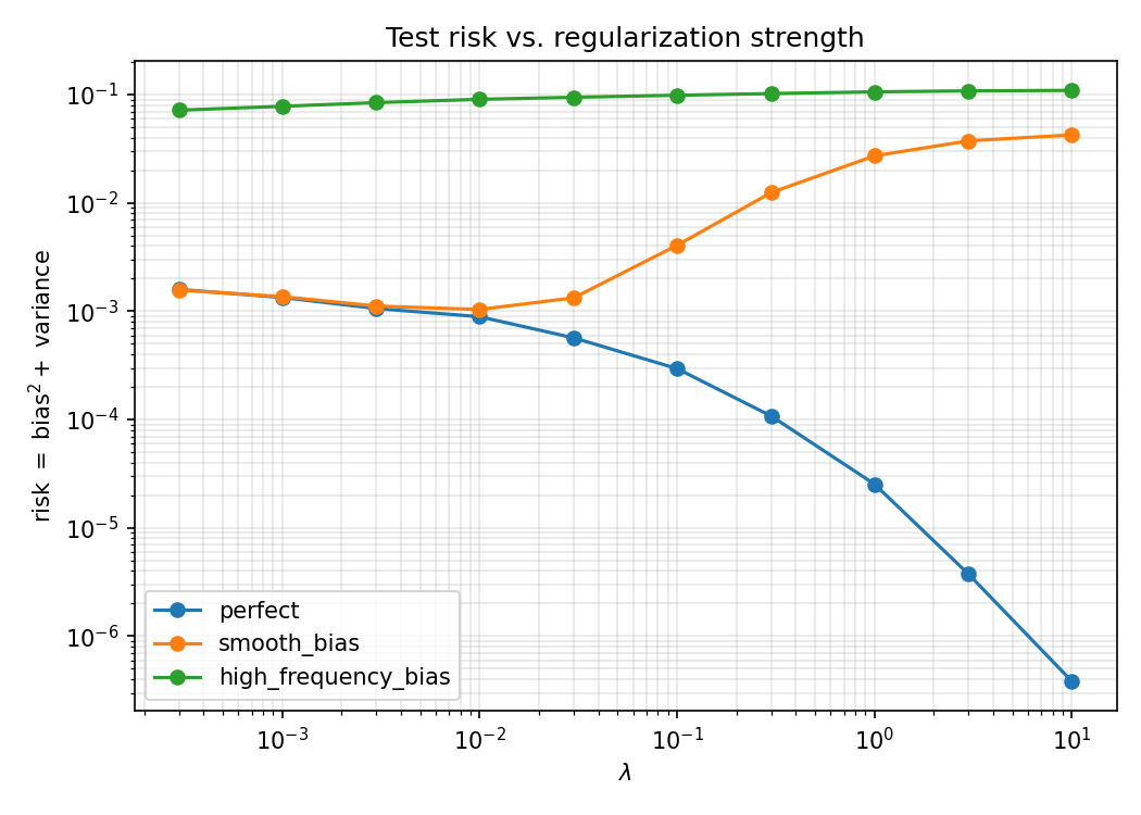
Perfect (monotone down), smooth bias (U-shaped, best near $\lambda\approx10^{-2}$), and high-frequency bias (high and flat) — the three regimes the theory predicts.